Learn how to make Pivot Tables, VLOOKUP, and absolute/relative formula references work harder.

I’m sure we’ve all been faced with the need to create a quick analysis/fishing expedition of some sort, and the first temptation is to go to Excel and create a Pivot Table, at which point we can hit some …frustrations.

This next example is fairly straightforward in nature, but hopefully shows that it is possible to squeeze a lot of information into a Pivot Table set up without taking up inordinate amounts of space and time.

It appears that there are a fair number of steps laid out below, but once you get a few under your belt it goes pretty fast.

Download companion Excel file*

Consider the following table:

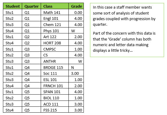
For example, going with ‘count’ in a Pivot…


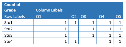
…we get a table that is factually correct, but not very enlightening. So, you can try an ‘Average’ calculation as well as pulling in ‘Class’…


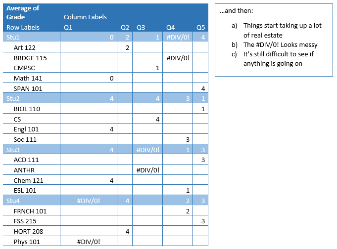
But if one could show the entries of Class and grade in the cells, rather than ‘just numbers’, like this:


…then I would argue that we have something that allows us to get quickly to a ‘feel’ for what’s going on with the students, their performance, and their attendance before going on (if deemed justified) to trying something more complicated with other tools. But how do we get here quickly?

This involves having Excel Pivot Tables, VLOOKUP and (optionally) the CHAR() function all work together to create row/column indexes to access cells in a predictable manner. In the Excel workbook (Sheet ‘Normal’) I start with a standard flat file and straightforward Pivot Tables to illustrate the frustration outlined above.

The ’Normal’ worksheet is where (in my experience) people tend to stop. But, with a little effort, a more condensed/readable set of tables can be created. 

The ‘PullingItAllTogether’ worksheet is intended to show everything in one fell swoop, with the ‘StepX’ worksheets breaking out the steps out in more detail.

STEP 1

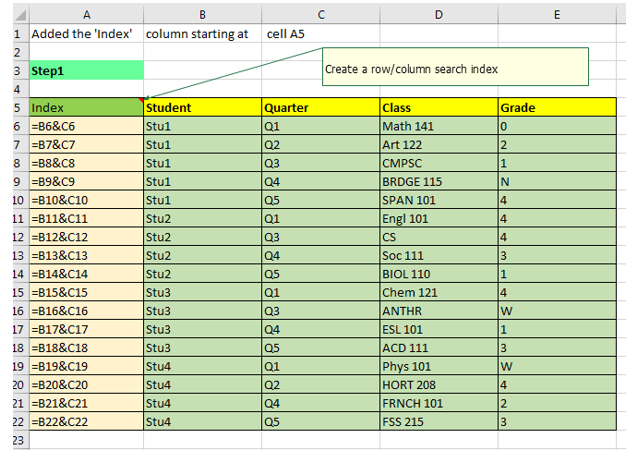
In this step I have added an ‘Index’ column to the data table that consists of concatenating the Student and Quarter fields (which will give me a Pivot Table cell position using Row and Colum references).

This table is then used to create a row/col Pivot Table for Step 2.

STEP 2

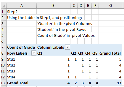
In Step 2 (in practice, this step can be skipped, but I wanted to try and show what was happening a little more clearly). The issue at this stage is that the ‘Count of Grade’ does not give us much information, and having letter grades present means we cannot calculate average grades. (or even show classes and grades ‘tidily’).

Which brings us to step 3 where I use the table in step 2 to help ‘re-interrogate’ the original table in order to bring in additional information without adding significantly to the amount of ‘screen estate’ being used.

STEP 3.1

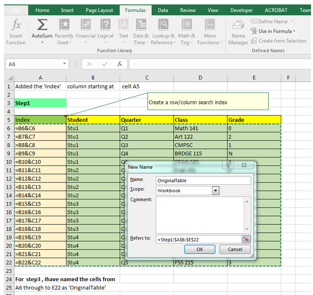
There are two stages here, one involving the ‘Step 1‘ worksheet. First, name your original table!

Just below I have named cells A6 through to E22 as ‘OriginalTable’ in the ‘Step1’ worksheet. (Note that I am on the ‘formulas’ tab, and that I got to the ‘New Name’ dialog box by selecting ‘Define Name’ in the top right hand side of the screen shot.) I find naming regions helps with readability/figuring out what you were thinking when you have to update the workbook after 6 months!


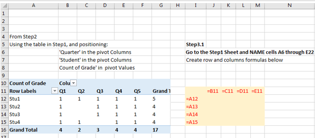
Then, in sheet ‘Step 3.1’ proper, I insert some basic row/column heading formulas (see below).

STEP 3.2

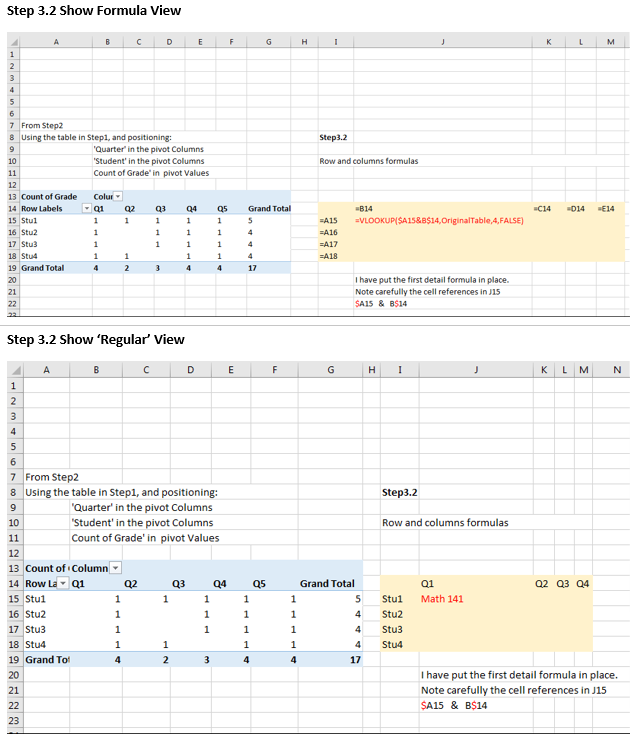
Now the fun begins. By using a combination of VLOOKUP and absolute and relative cell references, we can create a search key on the original table, using the Pivot Table as an aid. In cell J15 in the screen shot below, the formula concatenates the row and column headers of the Pivot Table to create a ‘Stu1Q1’ type reference that then searches the INDEX column (In the Step 1 sheet, in the ’OriginalTable’, and returns the 4th column entry from that table, which for J15 resolves to Math 141). Be careful to note the ‘$’ signs in the cell references in the formula.

STEP 3.3 & 3.4

To insert the grade, we extend the J15 formula by appending a “/” to the first VLOOKUP and then create a mirror of that first VLOOKUP by returning the ‘Grade’ (column 5) entry, which resolves to ‘Math 141/0.’


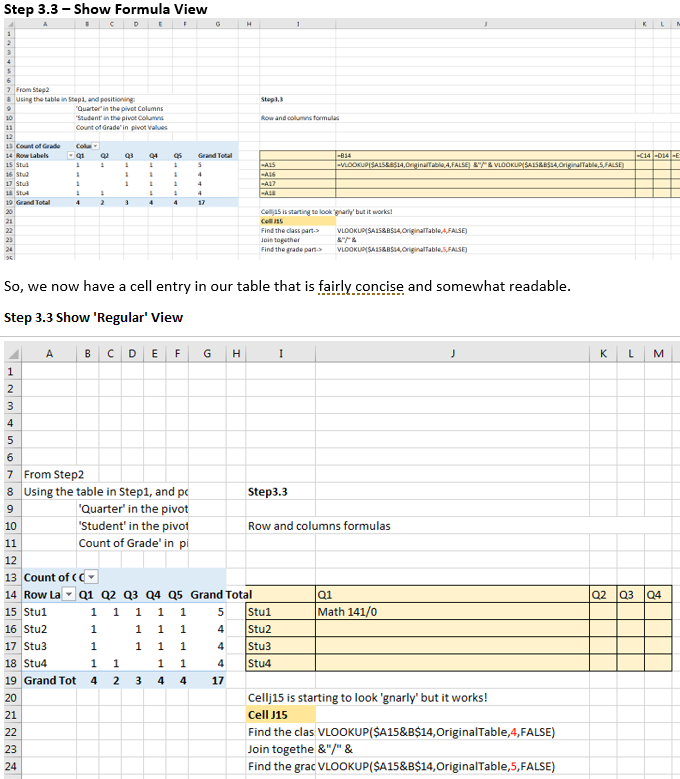
Now, if we take cell J15 and propagate across to cell M15, then down to M18, we get a bit of mess as shown below - but it’s solvable!

 

STEP 3.5

This last step inserts a ‘CHAR(10)’  into the formula to force a linefeed within the cell (providing  you also select ‘Wrap Text’ in the ribbon), in the event that you want detail data to appear on separate lines.




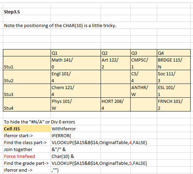
This table shows the results with the final formulas propagated. It could have perhaps been set up with Class/Grade on the top line of each detail cell with the whether the class was a repeat or not, online or face-to-face, and with instructor name on subsequent lines, but you probably get the gist of it.

While this explanation is lengthy, I think you will find this tip is quick to set up and hope you will see other areas for which to apply the technique! Have fun!

*For best results, in Internet Explorer, right-click on the link and choose "Save Target As" to save the file to your desktop.