The tidyverse is a set of tools in the programming language, R, for data wrangling, modelling, and visualization. There are a number of functions that allow data to be “read in” from multiple formats, transformed into a useful structure, and then visualized using the ggplot2 system. The syntax for the tidyverse is meant to assist even those with a limited programming background to be able to accomplish things quickly. I illustrated an example below using IPEDS data to examine national salary gender equity from 2005 to 2017 by rank. Two good books for those starting to learn R are included at the end of this tip. The most recent version of R can be downloaded from the Comprehensive R Archive Network and RStudio is also available.

IPEDS Salary Data

The analysis illustrated here could be a first step in institutional salary benchmarking or provide a set of input data for a salary equity study. All R code and source data are provided in a link at the end of this tech tip. A CSV file of faculty salary data by gender is available from the NCES IPEDS Data Center. I download this data from 2005 to 2017 for all title IV participating institutions in the US. Each row is a separate institution and rank. There are columns for IPEDS ID, institutional information, year, rank, full time faculty head counts by gender, and average salaries by gender.

The data has a small issue, however, in that only average monthly salaries are available for 2012-2016 by gender, whereas 9-month average salaries are available by gender from 2005-2011 and 2017. We can easily correct for this in our R script (shown later). I renamed the columns in each of the downloaded files to remove capital letters, introduced _ (underscore) in lieu of spaces, and shortened the variable names to remove the year.

Reading in the Data Files

This first step is to “read in” the files to my R environment.

The code above does several things. The first two library statements read in the tidyverse family of packages and the readxl library (which will help “read in” Excel documents). The next line creates a list of files located in the RawData directory that end in a .xlsx extention. The final line of code reads those files in, using the readxl library, and combines them using the tidyverse libraries. Because all the column names match in each data sheet, this can be automated. There would be issues if I didn’t name all column names the same (and I would need to have a line of code for each file, plus do some more wrangling before combining them).

Using the Data

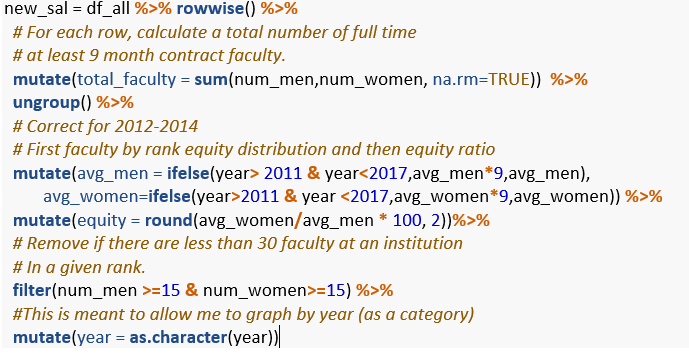
There are a few things we want to do with this data: first, we want to calculate a new variable representing the number of total faculty. Second, we want to adjust the data for 2012 to 2014 to be for a 9-month contract (as the original data was only available for monthly average by gender). Third, we want to calculate a gender equity salary ratio of average salary for women divided by the average salary for men times 100. After examining the data, we have decided to exclude data where the number of men and number of women are less than 15 for a given rank at an institution to allow for a more reasonable comparison of salary equity. This eliminates 66 percent of the rows in our original data set (from 144,843 observations to 50,152 observations over the 12-year period). The code below implements each of these decisions. In R, lines that start with a # are comments (and not actually run).

Once these transformations are completed, what can we do with the new data set? To explore salary equity nationally for the time period, we can summarize and plot the data.

The "summarize" step takes the grouped data by year and rank and for each combination of year and rank, calculates an Average Equity value, labeled AvgEquity. That is the weighted mean of the equity values in the data set where the higher amounts of faculty are weighted more and smaller are weighted less. I also calculate the standard deviation, labeled sd_equity, for each year and rank combination along with the total number of institutions that are represented by that combined data point. The final “mutate” verb takes (as an input) the original rank value and reorders it (this helps mainly for displaying the data).

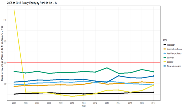
The above code performs the following actions: creates a plot in our Gender Equity summary by rank for each year, sets the labels and adds a line in bright red to represent salary equity, and defines and uses a color palette that is meant to be interpretable by people with color sight deficiencies.

Examining the above graph, two things become clear: first, there doesn’t seem to be much movement toward salary equity between men and women over the last decade, and second, something weird happened in 2005 with lecturers. I am a bit surprised by the first finding – while salary equity (at least for gender) in academia is better than reported for other sectors of the U.S. economy, there has been no major upward movement. The 2005 lecturer data, however, also seems striking. We can easily examine the data by filter on rank and year.

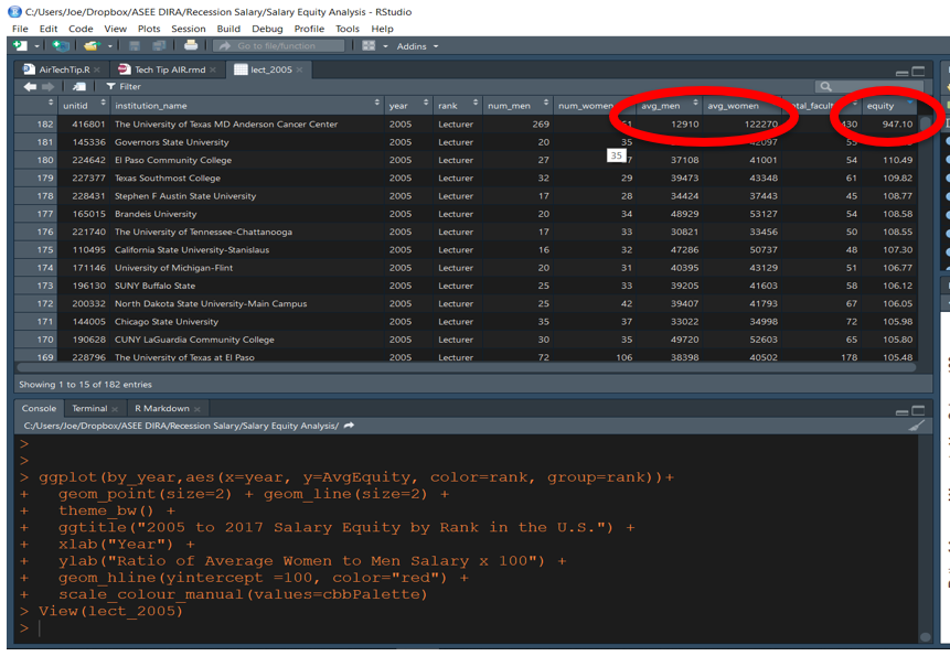
Within R Studio, I can sort the data set by equity amount and notice the problem immediately. A medical center probably misreported their data. While lecturers who are women have an average salary of 122k, lecturers who are men have a reported 9-month salary of 12k - which is a most likely a mistake.

The tools in R and RStudio allow for the scripting of data wrangling that lets an analyst document and iterate through different paths of exploration and report generation.

R Code

The code and data are available online.

Resource Books

1. Modern Data Science with R. 2017. Benjamin S. Baumer, Daniel T. Kaplan & Nicholas J. Horton.

2. R for Data Science: Import, Tidy, Transform, Visualize, and Model Data. 2017. Hadley Wickham & Garret Grolemund.