Predictive Analytics for Beginners

Predictive analytics has received quite a bit of attention in the professional literature on Institutional Research in recent years. For example, the fall 2023 volume of the AIR Professional File was devoted to predictive analytics and machine learning. Additionally, in the last few years, eAIR has published a number of short articles on various topics related to predictive analytics, including the value of faculty input on predictive analytics, and a comparison of the utility of using simple versus complex models when conducting predictive analytics (Mariani, 2021; Simpson, 2020; Utility of Simple vs. Complex Models, 2021).

Despite the attention that predictive analytics has received in the literature, what seems missing is a concise introduction to getting started with predictive analytics. Thus, this article seeks to fill that gap by providing a concise tutorial on how to conduct a predictive analytics study, and how to effectively present the results of such a study. This article will focus on the types of projects that small IR offices can easily undertake, as it will discuss how to conduct a predictive analytics study using commonly available software such as SPSS and Excel.

Background

The first step in conducting a predictive analytics study is to gather and analyze the existing data on the topic of interest. Since the ultimate goal of this first step is to produce an equation that describes the relationship between the dependent variable and the independent variable(s), multiple regression and logistic regression are frequently used introductory techniques (Lukan-Skinner and Shedd, 2020). Readers unfamiliar or needing a refresher on these topics are encouraged to consult Field (2017) or Kremelberg (2011).

After analyzing the existing data, the next step is to gather new data on the independent variable(s) of interest. For example, if analyzing the relationship between high school GPA, standardized test scores, and fall-to-fall retention in step one, step two might be to gather data on high school GPA and standardized test scores from recently admitted students. Then apply the new data to the equation developed in step one in order to predict which students are likely to persist from fall-to-fall. Predictive analytics is an iterative process in that adding new data to a model typically increases the accuracy of the predictions that are made. Thus, step three would be to add the new data to the model when it is available, which produces a new equation that describes the relationship between the variables. Subsequent efforts at predicting the variable of interest should be made with the model that best fits the data, which is typically the latest iteration of the model.

Example

In order to illustrate this process, the following section will discuss the steps I took to complete a predictive analytics project that was designed to predict student performance on the Step 2 Clinical Knowledge (CK) exam, which is a licensing exam that students take in their third year of medical school.

The project began with exploratory data analysis on historical data. The goal of this first step was to determine which variables were significant predictors of Step 2 CK performance. It was determined that in this dataset, race, gender, and pre-matriculation variables such as undergraduate GPA and standardized test performance were not significant predictors of Step 2 CK performance. However, it was determined that performance on the National Board of Medical Examiners “shelf” exams, which are standardized exams that third year MD students take after completing each required clinical clerkship, were significant predictors of performance on the Step 2 CK exam.

Since both the dependent variable (Step 2 CK score), and the independent variables (shelf exam scores for each discipline) were all continuous variables, ordinary least squares regression was an appropriate analysis technique. I conducted the regression analysis in SPSS, although one could use Excel if SPSS or another statistical software package was unavailable. Since there were about 1,000 cases available, all of the existing data on student performance on the Step 2 CK exam was analyzed. The results of the regression analysis are presented in Table 1.

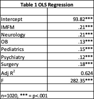
The regression analysis demonstrated that a student’s Step 2 CK exam score can be predicted using the following equation:

y = 93.82 + (.38 * IMFM) + (.42 * Neuro) + (.25 * OB) + (.28 * Peds) + (.33 * Surgery)^[1]

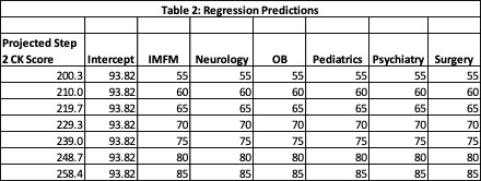
In the next step, an Excel worksheet was created in order to calculate predicted performance on the Step 2 CK exam based upon hypothetical scores on the shelf exams. This is illustrated in Table 2. At the time, a passing score on the Step 2 CK exam was 214, thus the calculations demonstrate that students need an average score in the lower sixties on the shelf exams in order to be predicted to pass the Step 2 CK exam. This was useful information for faculty advisors. Students take the shelf exams throughout the course of their third year in medical school and take the Step 2 CK exam at the end of their third year. Thus, based upon this analysis, faculty advisors began offering counseling and remediation to students that scored lower than 70^[2] on the shelf exams that they took early in their third year of medical school.

After I presented this portion of the project, the faculty advisors indicated that they were interested in examining not only an estimate of the students’ Step 2 CK scores, but also a confidence interval. They were also interested in receiving this information early in the year, before students had taken all of their shelf exams.             In order to accomplish this, I collected data on shelf exam performance from the current cohort of students after they had taken two or three shelf exams. I utilized Excel to calculate each student's predicted Step 2 CK exam score based upon their performance on the shelf exams using the equation presented above. Since students had not taken all of their shelf exams, I used their mean score on the exams that they had taken as an estimate of how they would perform on the remaining exams. The lower band of the confidence interval was calculated by multiplying the t-value (90% was selected) by the approximate standard error of the prediction, and subtracting the resulting value from the point estimate. The upper band of the confidence interval was calculated similarly, except the value obtained by multiplying the t-value and the approximate standard error of the prediction was added to the point estimate. The t-value can easily be calculated in Excel using the T.INV function.  In order to estimate the standard error of the regression predictions, the standard error of the regression model was multiplied by 1.1, as recommended by Armstrong (2001). Another option would be to calculate the standard error of the regression predictions using the appropriate formula (Montgomery et al, 2012, p. 52).

See Table 3 for an example of how to present the results of these calculations.

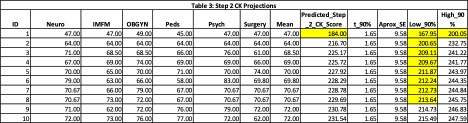
The faculty advisors found the results presented in Table 3 to be particularly helpful. They are able to monitor student performance on the shelf exams and offer counseling or recommend remediation to students that are performing poorly on the exams before the students are in a position to fail the high stakes Step 2 CK exam. Additionally, they found the confidence interval information to be extremely helpful when meeting with students that had yet to take the Step 2 CK exam, but were getting started with their residency applications. Residency in some fields is very competitive, and information on a student’s predicted Step 2 CK score is very helpful in guiding a student towards a program in which they are likely to be a competitive applicant.

Conclusion

Hopefully, this short introduction to predictive analytics has been useful to IR practitioners that are interested in getting started with predictive analytics but unsure as to where to start. When one realizes that predictive analytics is essentially an exercise in applied regression, predictive analytics seems much more approachable. Additionally, this article has demonstrated that many predictive analytics projects do not require significant technological resources to complete, and can be successfully undertaken using only commonly available software.