Whether you're new to Excel or breathe advanced formulae, there are always shortcuts and useful features to be discovered. Have you ever wanted a distinct count in pivot tables or an easier way to format complex workbooks? How about a quicker way to use your favorite actions?

You can transform your Excel experience. Keep reading for tips that have been learned through hard experience, diligent web searches, and gleaned from collaborative projects. 

Tip 1: Use Conditional Formatting to Highlight Duplicates
As there is no need to sort or alter your data, this is useful for quickly validating or checking data.

Select the cells/rows/columns/worksheets you want to check for duplicates. (This won’t check for an entire duplicated row though; each cell is compared to each other cell.)

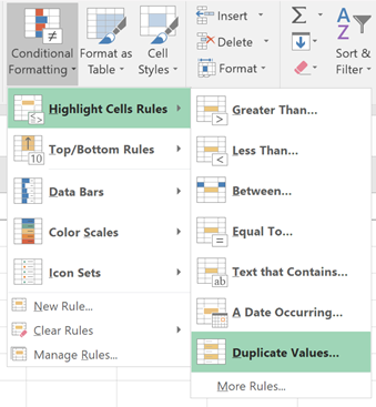
Then click the Conditional Formatting button and select Highlight Cells Rules and Duplicate Values.

If you want to use a specific color or format, select it from the prompt. Otherwise, just click OK.

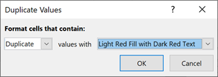
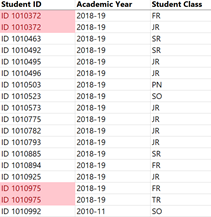
You can now see which cells are duplicated in your data! 

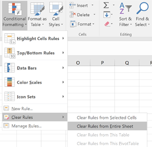
To clear the conditional formatting, go back to Conditional Formatting and choose Clear Rules. You can then clear just the currently selected cells, or everything on the entire worksheet.

Tip 2: Display a Distinct (Unduplicated) Count in Pivot Tables
So, you just discovered duplicates in your data but you need an unduplicated headcount for your report. Do you have to go back to the source, or remove them from your table? Many of us live in pivot tables, and yet this feature was so carefully disguised I'd never come across it until a colleague casually used it. And it's so easy!

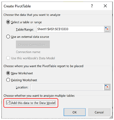
If you have duplicates in your data, but you don't want to remove them, just do one thing differently when you create your pivot table: check that little box that says Add this data to the Data Model. 

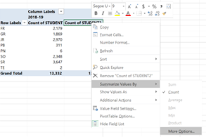
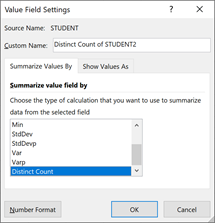
Then you’ll find the option for a Distinct Count under Summarize Values By and More Options. It’s hidden right at the end of the list.

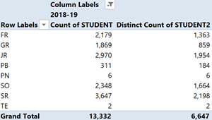
And now you have an unduplicated count!

One word of warning: you can’t group data within a pivot table if it’s using the Data Model. 

Tip 3: Customize your Quick Access Toolbar
This is found in the main title bar of Excel, up in the top left. 

If you haven’t used it because the default options are just save, undo, and redo, it’s time to rethink it. There are many other actions we use over and over, and you can add your favorites to this toolbar. Inserting pivot tables or charts, sorting or filtering data, highlighting duplicates, using text-to-columns, or creating PDFs are easy, but often take a few clicks or keystrokes. 

There are three ways to add them to your quick access toolbar.

1. A few actions can be added straight from the drop-down arrow on the far right.
   
   
2. You can also right-click anything in the ribbon and choose Add to Quick Access Toolbar. 
   
   
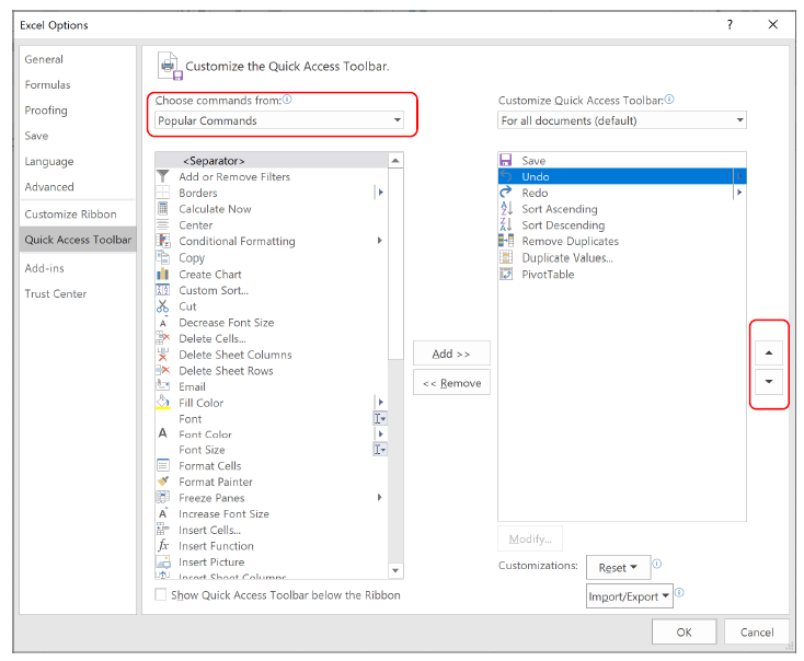
3. If you still can’t find what you want, go back up to the Quick Access toolbar and select More Commands.
   
   This is the most powerful option, but it can take some time to find some commands. Start by looking at what’s available. If you don’t see what you want, go back to the top drop-down (circled) and try looking at Commands Not in the Ribbon, All Commands, or Macros.
   
   Once here, you can also rearrange items in your Quick Access toolbar using the arrows on the right.

Tip 4: The Power of Groups
Have you ever been handed a huge workbook with multiple worksheets and been told, “This is now yours”? 

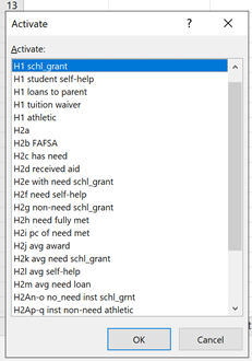
First, get an overview by right-clicking either of the navigation arrows in the bottom left corner down by the worksheet tabs to see a navigable list of all the worksheets.

If data has been exported from another system, you may need to make the spreadsheet more readable by removing header rows, creating consistent formatting, or setting all the column widths to auto-fit. This is where sheet groups come in. 

Sheet groups replicate changes across multiple worksheets, minimizing repetitive actions and letting you work more efficiently. Changes you make on one worksheet will be replicated on the rest of the group, whether that’s changing the font in A7, inserting a logo, setting column B to a percentage format, deleting row 54, or adding formulae.

To create a sheet group, hold down the Shift key and click the first and last sheet tabs. All sheets in between will become a group. You’ll notice that when you release the Shift key, the tabs are now temporarily white as a visual indicator.

You’ll also see [Group] appear after the filename in the title bar.

Now you have a group, you can set all the column widths to auto-fit in two actions. Select the entire worksheet, and double-click one of the columns as normal. That’s it!

If you want changes to apply to all the worksheets in a workbook, right-click one tab and choose Select All Sheets. You can also group non-contiguous worksheets, by holding down Shift and Ctrl before selecting the individual worksheets you want.

Some other uses for groups:

• Print all selected
• Move to the end/beginning
• Color code tabs
• Add a logo
• Delete a column with identifying information
• Hide unnecessary worksheets (remember that anyone can unhide them unless you lock and protect the workbook)

To ungroup sheets, simply select another tab that's not in the group. (If you prefer an explicit action, right-click on any sheet tab in the group and choose Ungroup Sheets.)

Tip 5: Control Your Work

There are many keyboard shortcuts built into Excel, and some of the most common use the Control (Ctrl) key. You probably already know about Ctrl-B (bold) or Ctrl-Z (undo) but how about these?

• Use Ctrl with the + (plus) key to insert rows, columns, or cells. Ctrl - (minus) will remove them.
• Ctrl-click the arrows to go to the first or last worksheet in a workbook.
• Hold down Ctrl and drag a worksheet tab to the right to duplicate it.
• Ctrl and ; (semi-colon) inserts the current date. Ctrl : (colon) inserts the current time.
• Ctrl and ‘ (apostrophe) copies the formula from the cell above.
• Ctrl and 9 (nine) hides selected rows. Ctrl and 0 (zero) hides selected columns.

These are just the tip of the iceberg, so to speak. If you want to explore more on your own, there are plenty of free resources for every level. Here are links to training from Microsoft and the Microsoft YouTube channel. Please comment to share your favorites with others in the AIR community.